Forced Vibrations

In the last section, we looked at springs and circuits subjected to damping, but not to any external force.  We now begin a discussion on vibration subjected to an external force.  We first consider the case where there is an external force but no damping.  We will also assume that the force is periodic and can be written as a cosine function.  We have

        mu'' + ku  =  F₀cos(wt)

From the last section we saw that the homogeneous solution is given by 

        y_h  =  c₁ cos(w₀t) + c₂ sin(w₀t)

There are two main cases to consider.  Either w  =  w₀ or w  w₀.  The two cases are profoundly different and an error in assuming one case while the other case can be catastrophic as we will soon see.

Case 1:  w  w₀

With this case, the UC-set does not coincide with the homogeneous set.  Hence a particular solution is given by 

        y_p  =  Acos(wt) + Bsin(wt)

After taking 2 derivatives substituting into the original equations and performing trig magic, we get

                          F₀
        y_p  =                           cos(wt)     
                    m(w₀2 - w₂)

If the mass starts at 0 and at rest then after much much more trig magic, we can arrive at 

                          2F₀                   (w - w₀)t                 (w + w₀)t
        y  =                           sin                         sin                         
                    m(w₀2 - w₂)                 2                              2

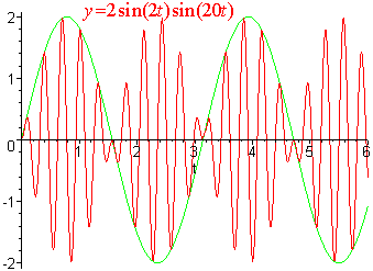
Although this looks like a mess that is incomprehensible, if we look at in the right way, the important  features of the graph will come clear.  If |w - w₀| is much smaller than w + w₀ we can think of 

                           2F₀                     (w - w₀)t  
       y   =                              sin                       
                      m(w₀2 - w₂)                   2        

as the "amplitude"  of the periodic function.  The amplitude is not a constant, but rather a periodic function itself.  This variation of the amplitude is called a beat (for sound) or amplitude modulation (for electronics).  You may recognize this better as "AM radio".  Below is a graph of a vibration with a beat.  The green curve is the graph of the amplitude  y  =  sin(2t)

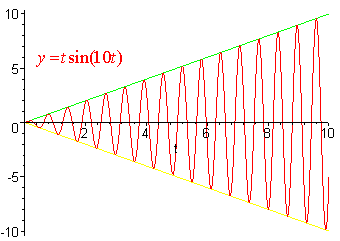
Case 2:  w  =  w₀

For this case, the UC-set coincides with the homogeneous solutions.  We must therefore multiply by t and get  

        y_p  =  Atcos(wt) + Btsin(wt)

Again, if we assume that the mass starts at rest at the origin, then after lots of algebra and trig magic, we arrive at

                                                            F₀   
        y  =  c₁ cos(w₀t) + c₂ sin(w₀t) +             t sin(w₀t)
                                                          2mw₀ 

This equation is markedly different from the "beat" equation.  Instead of the amplitude being periodic, it is linear tending to infinity as t tends to infinity.  This phenomena is called resonance.  In terms of design, the vibrations will reach a point at which the structure will be torn apart by the massive amplitude.  This was the cause of the collapse of the Tacoma Narrows Bridge. Click here for a video clip of this catastophe.  The frequency of the wind matched the length of the ends of the bridge.  Another example was when the space shuttle's turbo pump was accidentally designed with resonance structure.  Fortunately, the engineers notices the problem before take-off.  The error cost NASA millions of dollars.  For information on the space shuttle example go to http://www.fotuva.org/feynman/challenger-appendix.html.  Below is a graph of a vibration with resonance.  Notice the amplitude growing linearly.

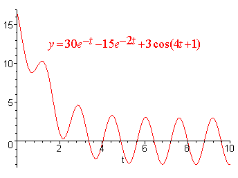
Forced Vibrations with Damping

For vibrations that have both damping and an external periodic force, the general  differential equation is given by 

        mu'' + gu' + ku  =  F₀cos(wt)

With a lot of work we can come up with the general solution.  We leave the details out and just state the result.  The solution is

        y  =  c₁e^r1t + c₂e^r2t + R cos(wt - d)

Where r₁ and r₂ are roots of the characteristic equation and R and d are constants that can be written in terms of the original constants.  If the roots are real, then they are both negative and if they are complex, then they have negative real parts.  In either case, the first two terms tend to zero as t gets large.  What this tells us is that the damping eventually erases the effects of the initial position and velocity, leaving only the effect of the forcing function.  The homogeneous solution 

        y_h  =  c₁e^r1t + c₂e^r2t 

is called the transient solution, since it goes away after awhile.  The particular solution 

        y_p  =  R cos(wt - d) 

is called the steady-state solution or the forced response.  The graph below shows an example of a typical solution.

Back to the Application and Higher Order Equations Home Page

Back to the Differential Equations Home Page

Back to the Math Department Home Page

e-mail Questions and Suggestions