Homogeneous Systems
In this discussion we will investigate how to solve certain homogeneous systems of linear differential equations. We will also look at a sketch of the solutions.
Example
Consider the system of differential equations
x'
= x + y
y' = -2x + 4y
This is a system of differential equations. Clearly the trivial solution (x = 0 and y = 0) is a solution. The origin is called a node for this system. We want to investigate the behavior of the other solutions. Do they approach the origin or are they repelled from it? We can graph the system by plotting direction arrows. We will calculate a few of these arrows and then use a computer to finish the plot.
Consider the point (0,1). We have
x' = 1 and y' = 4
so that
dy/dx = 4/1 = 4
We plot a small arrow emanating from (0,1) with slope 4.
Consider the point (1,0). We have
x' = 1 and y' = -2
so that
dy/dx = -2/1 = -2
We plot a small arrow emanating from (1,0) with slope -2.
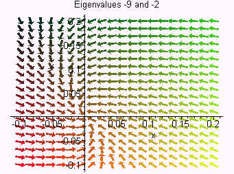
Below is a computer generated graph. We call the xy-plane the phase plane for the differential equation and the plot the phase portrait.
Notice that all solutions are repelled from the origin. The origin is called an unstable equilibrium point.
Our next task is to find an explicit solution for the system. We write the system as
x' = Ax
where
![]()
Just as with higher order differential equations, we assume that the solution is in the form
x = zert
where x is a vector solution and z is a constant vector. We have
x' = rzert
So that
rzert = Azert
We can divide by ert to get
Az = rz
Finding a solution is equivalent to finding an eigenvalue of the matrix. We can use a calculator to find that the eigenvalues are
r = 2 and r = 3
To find the constants, we can plug the eigenvalues into
A - rI
Plugging in r = 2 gives
![]()
The first row tells us that
-x + y = 0
and the eigenvector is
![]()
Plugging in r = 3 gives
![]()
The first row tells us that
-2x + y = 0
and the eigenvector is
![]()
We can conclude that the general solution is
![]()
or that
x = c1e2t + c2e3t
y = c1e2t + 2c2e3t
There is a direction relationship between the type of node the origin is and the eigenvalues of the matrix. In the example above the eigenvalues are both positive, thus both x and y are repelled from the origin as t becomes large. In particular if either of the eigenvalues are positive, then the trajectories repel from the origin. If the eigenvalues had both been negative, then both x and y approach zero as t approaches 0. Hence, all trajectories travel towards the origin for large t.
The cases where the eigenvalues are complex will be studied in the next discussion.
Back to the Power Series Methods and Laplace Transforms Home Page
Back to the Differential Equations Home Page
Back to the Math Department Home Page
e-mail Questions and Suggestions