Least Squares
Definition and Derivations
We have already spent much time finding solutions to
Ax = b
If there isn't a solution, we attempt to seek the x that gets closest to being a solution. The closest such vector will be the x such that
Ax = projWb
where W is the column space of A.
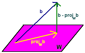
Notice that b - projWb is in the orthogonal complement of W hence in the null space of AT. Hence if x is a this closest vector, then
AT(b - Ax) = 0 ATAx = ATb
Now we need to show that ATA nonsingular so that we can solve for x.
Lemma
If A is an m x n matrix of rank n, then ATA is nonsingular.
Proof
We want to show that the null space of ATA is zero. If
0 = ATAx
then multiplying both sides by xT, we get
0 = xTATAx = (Ax)TAx = Ax . Ax = ||Ax||2
If the magnitude of a vector is zero, then the vector is zero, hence
Ax = 0
Since
rank(A) = n
we can conclude that
x = 0
We can now state the main theorem.
Let A be an m x n matrix or rank n, then the system
Ax = b
has the unique least squares solution
x = (ATA) -1ATb
Examples
Example
Find the least squares solution to
Ax = b
with

Solution
We can quickly check that A has rank 2 (the first two rows are not multiples of each other). Hence we can compute

Notice that

not exactly b, but as close as we are going to get.
Least Squares Regression Line
Of fundamental importance in statistical analysis is finding the least squares regression line.
ExampleAn engineer is tracking the friction index over mileage of a breaking system of a vehicle. She expects that the mileage-friction relationship is approximately linear. She collects five data points that are show in the table below.
| Mileage | 2000 | 6000 | 20,000 | 30,000 | 40,000 |
| Friction Index | 20 | 18 | 10 | 6 | 2 |
The graph below shows these points
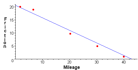
We are interested in the line that best fits the data. More specifically, if b is the vector of friction index data values and y is the vector consisting of y values when we plug in the mileage data for x and find y by the equation of the line, then we want the line that minimizes the distance between b and y. If the equation of the line is
ax + b = y
then we get the five equations
2a + b
= 20
6a + b = 18
20a + b = 10
30a + b = 6
40a + b = 2
The corresponding matrix equation is
Ax = b
or
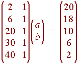
Although this does not have an exact solution, it does have a closest solution. We have

We can conclude that the equation of the regression line is
y = -0.48x + 20.6
Best Fitting Curves
Often, a line is not the best model for the data. Fortunately the same technique works if we want to use other nonlinear curves to fit the data. Here we will explain how to find the least squares cubic. The process for other polynomials is similar.
Example
A bioengineer is studying the growth of a genetically engineered bacteria culture and suspects that is it approximately follows a cubic model. He collects six data points listed below
| Time in Days | 1 | 2 | 3 | 4 | 5 | 6 |
| Grams | 2.1 | 3.5 | 4.2 | 3.1 | 4.4 | 6.8 |
He assumes the equation has the form
ax3 + bx2 + cx + d = y
This gives six equations with four unknowns
a + b + c + d = 2.1
8a
+ 4b + 2c + d = 3.5
27a + 9b + 3c
+ d = 4.2
64a + 16b + 4c + d
= 3.1
125a + 25b + 5c + d = 4.4
216a + 36b + 6c
+ d = 6.8
The corresponding matrix equation is
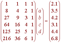
We can use the least squares equation to find the best solution
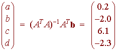
So that the best fitting cubic is
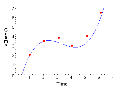
y = 0.2x3 - 2.0x2 + 6.1x - 2.3
The graph is shown below
Back to the Matrices and Vectors Home Page
Back to the Linear Algebra Home Page
Back to the Math Department Home Page
e-mail Questions and Suggestions