Solving Linear Systems of Equations

Reduced Row Echelon Form

When solving linear systems, we first transform the system into an augmented matrix.  At that point our goal is to transform the matrix into an "easier" matrix whose corresponding linear system has the same solution set.  We now defined what it means for a matrix to be "easier".

Definition

An m x n matrix is in reduced row echelon form if it satisfies the following properties:

1. All zero rows, if any, are at the bottom of the matrix
   
   
2. The first nonzero entry of each row is a one.  This one is called the leading one or the corner.
   
   
3. Each corner is to the right and below the preceding corner.
   
   
4. The columns containing a leading one have zeros in all other entries.

If only 1, 2, and 3 are satisfied, then the matrix is in row echelon form.

Example

Of the following three matrices, 

The A and B are in rref, while C is not.

The main purpose of putting a matrix in rref is that this form makes the solution of the linear system easy to identify.  For example A corresponds to the system 

        x₁  =  4        x₂  =  2        x₃  =  x₃ 

or in parametric form we get the line

        x₁  =  4        x₂  =  2        x₃  =  t

B corresponds to the system 

        x₁ + 3x₃  =  5        x₂ - x₃  =  0        x₃  =  x₃

This also gives us a line.  In parametric form it is 

        x₁  =  5 - 3t        x₂  =  t        x₃  =  t

Row Operations and RREF

We saw awhile back that the three row operation do not effect the solution space of a system of linear equations.  We restate the row operations here for convenience:

Three Elementary Row Operations

1. Switch any tow rows.
   
   
2. Multiply a row by a nonzero constant.
   
   
3. Replace a row by the sum of that row and a multiple of another row.

Two matrices are called row equivalent if one can be transformed into the other using a sequence of row operations.  Since row operations do not effect the solution space, any two row equivalent matrices have the same solution space.

Theorem

Every m x n matrix is row equivalent to a unique matrix in rref.

Instead of proving this theorem, we will explain how to take a matrix and transform it into an rref matrix using only the elementary row operations.  We follow the following procedures:

1. Switch rows (if necessary) to ensure that the top left entry is nonzero.  If the first column is all zero go to the next one.
   
   
2. Make this top left entry a 1 by dividing the row by this entry.
   
   
3. Use this 1 and the third row operation to zero out the entries below and above (there aren't any above for the first corner).
   
   
4. Repeat steps 1 through 3 for the columns to the right one at a time.

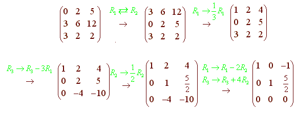
Example

Use the elementary row operations to put the following in rref.  

Solution

We follow the procedures:

Homogeneous Systems

A homogeneous system of linear equation is a linear system of equations where the right hand sides of all the equations are zero.  That is it is of the form 

        a₁₁x₁ + a₁₂x₂ + ... + a_1nx_n  =  0
        a₂₁x₁ + a₂₂x₂ + ... + a_2nx_n  =  0
          ...          ...                ...
        a _m1x₁ + a_m2x₂ + ... + a_mnx_n  =  0

Notice that in matrix form this can be written as

        Ax  =  0

where A is the m x n matrix with entries a_ij, x the the n x 1 matrix with entries x_i and 0 is the n x 1 zero matrix.  The augmented matrix's last column is the zero column.  Since the zero column is unaffected by elementary row operations, it is usually left out when the computations are performed.  The solution (0,0,   ... , 0) is called the trivial solution.  Any other solution is called a nontrivial solution.

Theorem

Let 

        Ax  =  0 

be a homogeneous system with m x n matrix A.  If m < n, then the system always has a nontrivial solution.

This theorem just states that if there are more variables than equations, then there is a nonzero solution.

Proof

Let B be the rref equivalent matrix to A.  Then B has a column that does not contain a corner.  This gives us a parameter in the solution which we can set to 1, giving us a nontrivial solution.  Since B has the same solution set as A, A has this same nontrivial solution.

Back to the Matrices and Applications Home Page

Back to the Linear Algebra Home Page

Back to the Math Department Home Page

e-mail Questions and Suggestions