Kenzie Ferguson          

Math 201

March 18, 2003

Math 201 Project

Introduction

This paper will discuss the differences between the real estate property sales in Palo Alto, CA versus Mountain View, CA and show that, on average, prices in Palo Alto are higher than in Mountain View. It would be appropriate for a potential homebuyer, seller, or real estate agent to use this report to gauge the price of a home in Palo Alto or Mountain View. To compare the real estate sales between Palo Alto and Mountain View a cluster sample of 6,298 real estate property sales were gathered from the years 1996 to 2002. The data on real estate sales were taken from the Palo Alto Weekly online real estate section.

Results

The following information was complied from the Palo Alto Weekly online Real Estate section (see appendix). A total of 6,298 real estate property sale prices were used to compile the 7 paired yearly averages. In Table 1, the years 1996 to 2002 are listed along with the average sale price of real estate property in US dollars for Palo Alto and Mountain View.

Table 1 Average House Sales in Mountain View and Palo Alto from 1996 to 2002.

Trimmed Mean

In order to exclude any outliers in the sample a trimmed mean is used to show a more reliable number for the sample. The data for each year was trimmed at 5%.

Table 2 Trimmed Mean of house sales in Mountain View and Palo Alto from 1996 to 2002

As you can see in comparison of data in table 1 and 2, the home sales decreased overall, with exception of homes in Palo Alto in 2001, leading us to believe there were very large outliers in the data collected.  

Summary statistics

The Student’s t variable is used to find the confidence intervals for each individual data set. The degrees of freedom for both sets is 7-1 = 6 and the level of confidence is 95%, which gives us the t_c value 2.447.

Palo Alto            E = 2.447(194,544√7)

                          E = 179,930

Mountain View E = 2.447(110,741√7)

                          E = 102,422

The population of Palo Alto property sales at a 95% confidence interval range from $492,365 to $852,225. The population of property sales in Mountain View at a 95% confidence interval range from $301,523 to $506,366.

The population of property sales in Palo Alto and Mountain View is approximately normal because, according to the Central Limit Theorem, the probability sampling distribution for the sample mean x of average property sales based on random samples of size n is approximately normal.

Central Limit Theorem: if x possesses any distribution with mean m and standard deviation s, then the sample mean x based on a random sample of size n will have a distribution that approaches the distribution of a normal random variable with mean m and standard deviation s/√n as n increases without limit.

Box-and-Whisker Plots

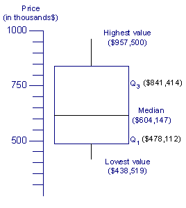
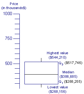
It may be important to our homebuyer to see the spread of property sales when making a decision about buying a home. If the buyer is looking for a home in the lower end of the range he may choose one city over the other. According to our data the median property sold in Palo Alto is $604,147 and the median house sold in Mountain View is $386,685. It will please our homebuyer that the median property sale is lower than the mean. This would cause us to believe that there are more homes in the lower range. 

The difference in sales prices is more pronounced in the Box-and-Whisker plot diagram. The interquartile range of the property sales in Mountain View is almost entirely below the interquartile range of the property sales in Palo Alto. If the buyer is interested in homes below $525,000 he would have a wider selection in Mountain View than in Palo Alto.

Frequency Distributions and Histograms

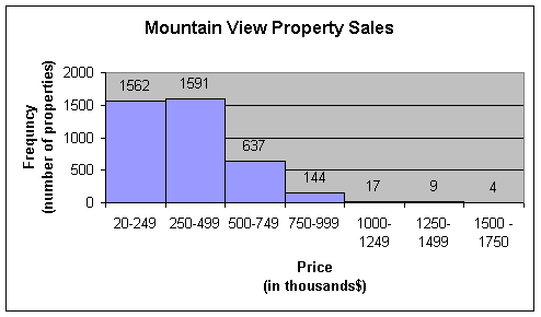
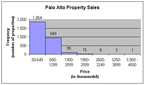
In order to get a better idea of the number of properties in a given price range we created a frequency table and graph for Mountain View and Palo Alto property sales.

Table 3

In the third column of Table 4 is the relative frequency. The relative frequency shows the percentage of properties in the class. In the Mountain View table 70.54% of the properties were sold in the combined $250,000 to 499,999 and $20,000 to $249,000 ranges.

Both of the following frequency histograms are unimodal and skewed right.

Paired Data Hypothesis Test

We have a sample of 7 years and the pair of measurements taken from the respective cities. The sample size is n=7 pairs, and the d values are found in the fourth column of Table 5. We find the sample mean  = 268,351 by summing the fourth column and dividing it by n = 7 and the standard deviation s_d= 86,455.

Table 6

First we will test the mean of the differences of paired data values. We will challenge the null hypothesis for the paired data: H₀: μ_d = 0. Because we are trying to prove that property sales in Palo Alto are higher than in Mountain View we will try to prove an alternate hypothesis, H₁: μ_d > 0. A right-tailed test is used and the level of significance is 5%: α = 0.05.

The right-tailed critical value, t₀ = 3.707, is found using the Student’s t distribution and the degrees of freedom: 7-1 = 6. The sample statistic d is converted to a t value using n=7;  = 268,351; s_d= 86,455; μ_d = 0 from H₀. The formula for paired differences d is used.

t = 268351 – 0 / 86455/ √7

  = 8.21

See Figure 1. Since the sample statistic falls in the critical rejoin, we reject H₀ at the 5% level of significance.

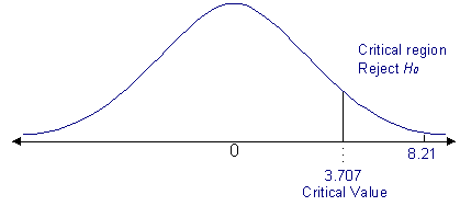
Figure 2

Hypothesis Test on the Slope

In order to better predict the relationship between the cost of a house in Palo Alto and that of one in Mountain View a hypothesis test on the slope is used.

H₀: r = 0; H₁: r ≠ 0.  

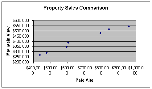
First we make a scatter diagram for these pairs. The x value is the average property sale in Palo Alto and the y value is the average sale in Mountain View paired by year. In general as the prices in Palo Alto go up the prices in Mountain View go up. There seems to be a relatively linear progression and a line fits reasonably well.

Figure 3

To find out the slope and the strength of the relationship between the two cities’ property sales we start by using the formulas to find the values of a and b.

Table 7

The sums in the table are used to compute the formula for the least-square line.

The least squares line for the data is

y = a + bx

y = 25,263 + 0.56x

The least-squares line is plotted on the scatter diagram with points (672,295.42, 403,944.45) and (500,000, 305,263).

Figure 4

Linear Correlation Coefficient

Finally, we need to test for linear association between the average property in Palo Alto and Mountain View. To find the correlation coefficient r we must look at the linear correlation. Figure 5 shows a positive linear correlation between Palo Alto and Mountain View property sales.  We arrive at r = 0.989 by using the formula to calculate the correlation coefficient, r. Because r is very close to 1 the Palo Alto and Mountain View property sales have a positive correlation and are nearly all points lie on the least-squares line. High-priced property sales in Palo Alto are associated with high-priced sales in Mountain View, and low-priced sales in Palo Alto are associated with lo-priced sales in Mountain View.

r² =0.979155801 means that 98% of the variation of y, the amount of the average property sale in Mountain View, can be explained by the least-squares line. The remaining 100 – 0.98 = 2% of the variation of y is due to random chance or other variables besides x, the amount of the average property sale in Palo Alto, that influence y.

Confidence Interval

With this equation a potential homebuyer can predict how much less a home in Mountain View will be in comparison to Palo Alto. For instance, a homeowner wants to sell their Palo Alto home for 500,000 and buy a home in Mountain View. The approximate amount the homeowner would be able to buy an average home in Mountain View would be $305,263 ± $705,783 with a 95% confidence interval.

The standard error of estimate for this least-squares line is

Se = √SSy – bSSxy/ n-2

Se = 243251.9

Conclusion

We have proven that, on average, prices in Palo Alto are higher than in Mountain View. A potential buyer would be able to use this information in making an informed decision when buying a home. In a situation where a Palo Alto homeowner sells their property and buys a home in Mountain View there is a good chance that the individual will be able to buy a house at a lower price. When a new buyer wants to enter the real estate market he can be confident that a home in Mountain View will, on average, cost less then in Palo Alto. This sort of information can be helpful in making a decision but is not the only variable to look at when buying a home.

Appendix

REM Reports Inc., a Walnut Creek real estate information company, originally compiled home sales prior to June 1997. Since then homes Titletech, and Oakland real estate information company originally compiled sales. Sale prices are estimated from the county transfer tax. Information is recorded from deeds after the close of escrow. The month reported from the search is up to four months after the close of escrow.

See attached Excel document for list of raw data.