STAT 201 PROJECT: CUSTOMER COUNT IN A CONVENIENT STORE FOR YEAR 2002 AND 2003 IN OCTOBER………………………..BY:KINJAL. PATEL

                                                                                                                            FALL 2003

Introduction:

This paper will discuss the differences in customer count in a convenience store for the month of October for the year of 2003 versus that of 2002. As the business is in Lake Tahoe is dependent on tourists it gives us an idea about what to expect in a particular month. Also it helps in staffing, whether to have more staff for a particular day or not. This also helps to see if the business has grown or shrunk as compared to last year.

Data:

The data was collected from a convenient store in Lake Tahoe for the month of October 2002-2003 by cluster sampling, as all the days for October are included. The data is quantitative, bivariate and continuous. This data is at the ratio level of measurement.

 The following tables show the statistics for customer count in Oct 02 and Oct 03.The trimmed mean for both the data is same as their mean , as there are no significant outliers.
Summary statistics for Oct 02

Summary statistics for Oct 03

Histograms

The Histogram for the customer count in Oct’ 02, shows that the data is Unimodal , skewed right

The Histogram for the customer counts in Oct’ 03, shows that the data is Multimodal with gaps in between.

Stem and Leaf Diagram:

Variable: C.COct02       Variable: C.COct03

Low: 10                              6: 3344           

 6: 0                                    6: 5678

 6: 88                                  7: 000122234

 7: 000011234444              7: 6889       

 7: 66778                            8: 14

 8: 1234                              8: 5579

 8: 556                                9: 0

 9: 03                                  9: 6

 9: 6                                   10: 

10: 1                                  10: 6

                                            High: 1095

Box and Whisker Plot:

                        Oct02      Oct 03      

It may be important for our store owners to know what the customer count is for a particular month to predict the sales. We can find this out by the box and whisker plots.

The box and whisker plot for the customer count in Oct’ 02, has the median more towards the center. The whiskers are evenly distributed in the top and bottom part. There is no outlier for this plot. IQR=Q3-Q1=838-707=131.

The box and whisker plot for the customer count in Oct’ 03, has the median more towards the lower part, indicating that more customers are in the lower half. There is also an outlier which affects the Q-2 value. IQR=Q3-Q1=845-683=162

Central Limit Theorem: If x possesses any distribution with mean m and standard deviation s, then the sample mean x based on a random sample of size n will have a distribution that approaches the distribution of a normal random variable with mean m and standard deviation s/√n as n increases without limit.

Hypothesis test for Paired Data
Two Sample Z-test results:
m₁ - mean of C.COct02
m₂ - mean of C.COct03
H₀: m₁ - m₂ = 0
H_A : m₁ - m₂ < 0

This shows that it is a left tailed test .The critical value for z-score for a left tailed test at 5% level is -1.645.

 For 95% confidence interval the range for the population mean m is

x-E<  m < x+E=[6.709-27.05,6.709+27.05]=[-20.34,33.76](read x as x-bar, sample mean)

  This means, that we are 95% confident that the average customer count for any given day is different as the range consists of both positive and negative values.

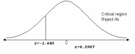
The z-score for the difference of mean is 0.25, therefore for the left tailed test

     P (z<0.25) =0.5987(from z-score table for left tail) which does not fall in the critical region

Also, p = 0.598 > α = 0.05

 Therefore, fail to reject H₀

 We do not have sufficient evidence at 5% level to indicate that the average customer count for the month of October 2002 is less than that of October 2003

Hypothesis Test on the Slope

In order to better predict the relationship between the customer count in the month of October ’02 and that of the count in October ‘03 a hypothesis test on the slope is used.

H₀: r = 0;

 H₁: r ≠ 0.  

First we make a scatter diagram for these pairs. The x value is the average customer count in October ‘02 and the y value is the average customer count in October ‘03 paired by dates.

In general as customer count in October ‘02 goes up customer count in October ‘03   go up. There seems to be a relatively linear progression and a line fits reasonably well.
Simple linear regression results:
Dependent Variable: C.C October 03
Independent Variable: C.C October 02
Sample size: 31
Correlation coefficient: 0.6703
Estimate of sigma: 90.32325

The least squares line for the data is

y = a + bx     , where a= 88.63   and b= 0.877

y = 88.63 + 0.877x

r=0.67

r²=0.45

Therefore, 45% of the variation in y can be explained by the variation in x. About 55% of the data is unexplained by the variation in x.

There is positive correlation between the customer count for the month of October 2002 and October 2003.

Chi -Test for independence of C.C October 02 and C.C October 03:

H₀: The Customer Count for October 2002 and 2003 are independent

H₁: The Customer Count for October 2002 and 2003 are not independent

χ² = 806

χ²_α > 140 ( for degrees of freedom 780 , from chi- square   table)

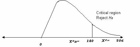
  As, the chi- square value falls in the critical region, we Reject H₀ .

We, have sufficient evidence at 5% level that the Customer Count for October 2002 and 2003 are not independent. ,but dependent. This means that with every increase in the Customer count in 2002 for each day, we can predict that there will be increase in 2003.

Conclusion:

We performed various tests and from the results we can conclude the following things:

        On an average the customer count of October 2002-2003 are different (difference on means).This shows whether the business has grown or shrunk from last year. This gives an idea as how to budget the expenses for the business

        As the count increases in October ’02 we can expect an increase in October ’03 too (Regression line). This information gives us an idea on how to staff on the slow days and busy days.

        The Customer Count in October’03 is dependent to that of October’02. (Chi-square test).

    This data and the results can be used by the store owners for their future interpretations of the Customer count, expected sale and staffing issues. Also a potential business buyer can look at the statistics to see how the store is performing, from the profit point of view.

Appendix:

    The data was collected from a convenience store located in South Lake Tahoe. Attached is the data that was collected: