Jason St. Clair

Mat 201 Project

3-17-2003

Stress at Harrah’s/Harvey’s

            Almost everyone deals with stress at work and at home. The perception is that the stress at work is much greater that the stress at home, very often you here someone complaining about a bad day at work. On the other hand you rarely hear complaining when somebody is stressed out at home. In this project I took a simple random sample of 46 employees of Harrah’s/Harvey’s and asked them two separate questions each, both dealing with their perceived level of stress. The first question was what was there perceived level of stress at work, and the second question was what was their perceived level of stress at home; both of these questions were on a scale of 1 to 10 with ten being the highest. I will show that the stress at work is higher than the stress at home. Therefore the difference of the Not Hypothesis and the Null will be different. The difference will not be the same.

H0: m1-m2=0   where m1 = mean of stress at work and m2 = mean stress at home.                   

H1: m1-m2 ñ 0

My second hypothesis is that employee’s stress level is higher at work than at home

H0: r = 0                

H1: r á 0

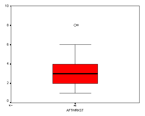
The mean for stress after work was 3.1957, this means that the average stress after work for the 46 people sampled around 3. The 5% trimmed mean was also around 3; this means that there really weren’t any big outliers around the top 5% and bottom 5% of the respondents. The 95% confidence interval for the mean was 2.7 and 3.6. The 95% confidence interval is used because there is not a definitive way that we can come up with the mean; therefore we use the 95% confidence interval to say that with 95% confidence the mean is within these 2 numbers. The median, which is the average of the middle most numbers, was 3. The standard deviation, which is the average distance between the respondent’s numbers, was approximately 1.6. The interquartile range, which is used for when the data is divided up into 4, sections called quartiles. The inter quartile range for stress at home was 2.

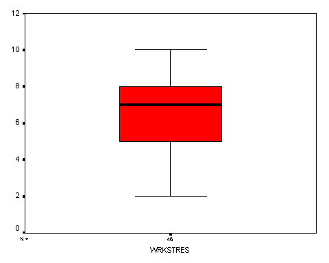
The mean stress while during work was 6.5870; the 95% confidence interval for the data was between 6 and 7.1. The median for the stress while at work is 7. The standard deviation was 1.95, and the Interquartile range was 3.

I also used stem and leaf plots to show where the respondents answered most of their questions, or what level of stress was perceived the most. In the stress not at work, the respondents answered 2 and 4 the most often. In the work stress survey 7 and 8 appeared the most frequent.

Box plots were also used to show where the greatest amount of the respondents answered their stress level. By looking at the Box plots it is clear to see that the perceived stress level is higher at work than the perceived stress level at home.

My paired data samples test proved that the difference between the means is 3.39 the standard deviation was 2.52, with a 95% confidence interval of 2.64 to 4.14 with a margin of error of ±. 37, this shows that the mean of work stress is higher. So we can conclude that we reject H0 and accept H1, the mean of the work stress is higher that the mean of stress at home.

My one sample T-test work stress mean was 6.58 with a 95% confidence interval of 6 to 7.1, the stress at home mean was 3.19 with a 95% confidence interval of 2.72 to 3.6. By looking at this data I can prove that my in my second hypothesis test that

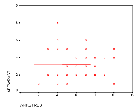
My regression line was relatively straight; my R square came out to be zero. This means that this regression line is a useless indicator for predicting the Y values. My regression line equation is y = 3.284 + -.013 (x). This is a negative correlation, and it is very weak because my R is very close to zero.

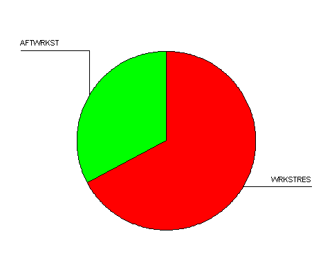
This pie chart show that the perceived stress level of the respondents is higher at work than at home.  My histograms show which stress level occurred most frequently, both of the histograms are non symmetric.