Aaron Molloy
Statistics 201
3/18/03
January Precipitation: Heavenly Valley and Vail Mountain
Precipitation can come in the many forms. There are times where the temperatures are below the freezing mark and a place can get large amounts of snow and there are times where the temperatures are above the freezing mark and an area gets rain. In the end, this study looks are precipitation in both forms. The data that was used in this paper was obtained from The National Water and Climate Center’s web page (www.wcc.nrcs.usda.gov). The Water and Climate Center is a branch of the U.S. Department of Agriculture. The data I used was historical precipitation data measured in inches. The sampling technique that I used was cluster sampling because the amount of precipitation was recorded daily and I chose to use everyday in the month of January in four separate years (n=124) from two areas of the United States. I chose Heavenly Valley in California and Vail Mountain in Colorado. I chose to use data from 1988, 1998, 2002, and 2003.
The null hypothesis in this project is that the mean amount of precipitation in Heavenly Valley is equal to the mean amount of precipitation in Vail Mountain. The alternative hypothesis is that the mean amount of precipitation in Heavenly Valley is greater than the mean amount of precipitation on Vail Mountain. The second null hypothesis and the main idea of this paper is that the amount of precipitation on Vail Mountain is independent of the amount of precipitation in Heavenly Mountain. The other alternative hypothesis is that the amount of precipitation on Vail Mountain is dependent on the amount of precipitation in Heavenly Valley.
The first calculations that I want to report are my descriptive statistics for both Heavenly Valley and Vail Mountain. (See chart below)
|
|
|
Statistic |
Std. Error |
|
|
HEAVENLY |
Mean |
1.1613 |
.17791 |
|
|
| 95% Confidence Interval for Mean |
Lower
Bound |
.8091 |
|
|
| Upper
Bound |
1.5135 |
|
|
|
| 5%
Trimmed Mean |
.8871 |
|
|
|
| Median |
.0000 |
|
|
|
| Variance |
3.925 |
|
|
|
| Std.
Deviation |
1.98116 |
|
|
|
| Minimum |
.00 |
|
|
|
| Maximum |
10.00 |
|
|
|
| Range |
10.00 |
|
|
|
| Interquartile
Range |
2.0000 |
|
|
|
| Skewness |
2.125 |
.217 |
|
|
| Kurtosis |
4.743 |
.431 |
|
|
VAIL |
Mean |
1.0565 |
.11526 |
|
|
| 95% Confidence Interval for Mean |
Lower
Bound |
.8283 |
|
|
| Upper
Bound |
1.2846 |
|
|
|
| 5%
Trimmed Mean |
.9158 |
|
|
|
| Median |
1.0000 |
|
|
|
| Variance |
1.647 |
|
|
|
| Std.
Deviation |
1.28343 |
|
|
|
| Minimum |
.00 |
|
|
|
| Maximum |
6.00 |
|
|
|
| Range |
6.00 |
|
|
|
| Interquartile
Range |
2.0000 |
|
|
|
| Skewness |
1.488 |
.217 |
|
|
| Kurtosis |
2.114 |
.431 |
|
In looking at this data we can see that the mean amount of snow for Heavenly Valley is 1.1613 inches/per day with a standard deviation of 1.98116 is greater than Vail Mountain’s 1.0565 inches per day with a standard deviation of 1.28343. Based on the empirical rule 68% of the days received between zero inches and 3.14 inches of precipitation. 95 % of the days received between zero inches and 5.12 inches of precipitation. 99% of the days where precipitation levels were measured received between zero inches and 7.1 inches. In looking at the standard deviation for Vail Mountain one can see that one standard deviation to the left is going to be a negative number. This just means that one, two, and three standard deviations to the left are going to be zero. It shows that 68% of the days received between zero and 2.34 inches of precipitation, 95% of the days received between zero inches and 3.62 inches of precipitation and 99% of the days received between zero inches and 4.90 inches of precipitation. The 5% trimmed mean for Heavenly Valley is 0.8871 and the 5% trimmed mean for Vail Mountain is 0.9158. This shows that when you delete the bottom 5 % of the data and the top 5% of the data then Vail Mountain gets more precipitation on average than Heavenly Valley. The median for Heavenly Valley is 0.000 inches of precipitation and the median for Vail Mountain is 1.000. This shows that the central value in the ordered distribution for Heavenly Valley is 0.0000 and the central value of the ordered distribution for Vail Mountain is 1.000. The maximum amount in inches that Heavenly Valley received in any given day is 10 inches and the Vail Mountain is 6 inches. Both of the areas received at least one day of no precipitation. The interquartile range is both 2 inches for Heavenly Valley and Vail Mountain. This tells us that the spread of the data between the third and first quartiles is both relatively small, but the same.
Below is a histogram of the amount of precipitation versus the number of days Heavenly Valley received each amount.
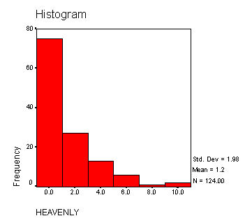
This histogram is unimodal and skewed right. It is clear from this histogram that the mode for Heavenly Valley is between 0.000-1 because it occurs most frequently and because the bar for the interval 0.000-1.000 extends the highest. .
Below is a histogram of the amount of precipitation versus the number of days Vail Mountain received each amount.
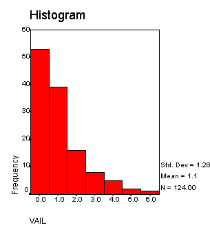
This histogram is also unimodal and skewed right. It is clear from this histogram that the mode for Vail Mountain is 0.000 because it occurs most frequently and the bar extends the highest in the histogram.
The next graph that I chose to use to display my data is called a stem and leaf diagram. This display allows me to organize my data, but also allows me to recover my original data points if needed. Below is the stem and leaf diagrams of both Heavenly Valley and Vail Mountain.
HEAVENLY Stem-and-Leaf Plot
Frequency
Stem & Leaf
75.00 0 .
0000000000000000000000000000000000000
.00 0 .
17.00 1 .
00000000
.00 1 .
10.00 2 .
00000
.00 2 .
4.00 3 .
00
.00 3 .
9.00 4 .
0000
9.00 Extremes (>=5.0)
Stem
width: 1.00
Each
leaf: 2 case(s)
VAIL
Stem-and-Leaf Plot
Frequency
Stem &
Leaf
53.00 0 .
00000000000000000000000000
.00 0 .
39.00 1 .
0000000000000000000
.00
1 .
16.00 2 .
00000000
.00 2 .
8.00 3 .
0000
.00 3 .
5.00 4 .
00
3.00 Extremes (>=5.0)
Stem
width: 1.00
Each
leaf: 2 case(s)
In the displays above one can see that the stem and leaf shows each data point and it also gives the frequency of the number of data points. These particular stem and leaf diagrams breaks the digits of each value into the ones digit being the stem and the tenths digit being the leaf. One other unique aspect of this diagram is each leaf stands for two data points. Again one can see that frequency that Heavenly Valley and Vail Mountain will get 0.000 inches of precipitation is far greater than them receiving even one or two inches of precipitation.
The next display I chose to use is called the box and whisker plot. Below I have included the box and whisker plots for both Heavenly Valley and Vail Mountain.
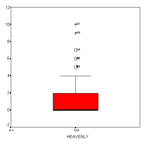
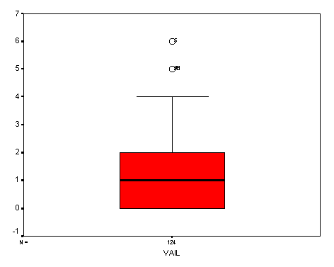
These box and whisker plots displays Heavenly Valley’s median is 0.000 and Vail Mountain’s median is 1.000. We see that the interquartile range is 2 inches in each and the whisker extends up to the highest value that has more than one data point and then beyond that the individual data points represent one day where that particular amount precipitation fell. Thus, we see that the maximum amount of precipitation that occurred on any given day for Heavenly Valley is 10 inches and for Vail Mountain is 6 inches.
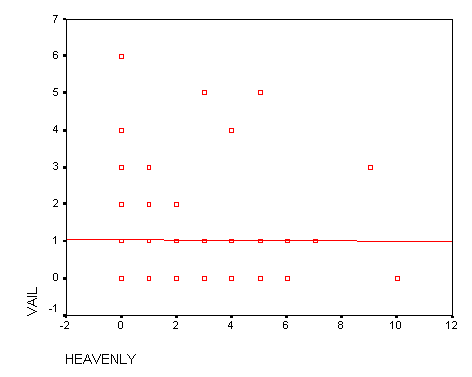
The following display of the paired data is a scatter diagram. I have chosen to view this scatter diagram with Heavenly Valley being the independent variable (X) and Vail Mountain being the dependent variable (Y).
Model Summary
|
Model |
R |
R Square |
Adjusted R Square |
Std. Error of the Estimate |
|
1 |
.007(a) |
.000 |
-.008 |
1.28865 |
a Predictors: (Constant), HEAVENLY
In looking above one can see that the best-fit line could be hard to draw because there is no linear correlation in the points. Above is a chart that shows that R squared is 0 and thus this line is not a good predictor of variation. This explains that 0% of the variation of Vail Mountain’s precipitation can be explained by the corresponding variation of Heavenly Valley’s precipitation. This r squared values tells me that 100% variation of Vail Mountain is do to other factors rather than the precipitation in Heavenly Valley.
|
Model |
|
Unstandardized Coefficients |
Standardized Coefficients |
T |
Sig. |
|
|
| B |
Std. Error |
Beta |
| ||
| 1 |
||||||
|
(Constant) |
1.062 |
.134 |
|
7.906 |
.000 |
|
|
| HEAVENLY |
-.004 |
.059 |
-.007 |
-.075 |
.940 |
a
Dependent
Variable: VAIL
The chart above gives us our a and b values for our least-squares line. The letter a is the y-intercept and the letter b is the slope of the line. The equation for our least squares line is:
Y= -.004 + 1.062X
This equation shows that for every additional inch of precipitation that Heavenly Valley gets Vail Mountain gets 1.062 inches more on the average. We can also interpret this equation to say that if Heavenly Valley gets no precipitation then the line predicts that Vail will get .004 inches. The Sig. Value is .940, which is really high, and thus this line is a useless indicator because a typical p value is .05.
The following charts represent the Paired samples test.
Paired Samples Test
|
|
Paired Differences |
|||||
|
|
Mean |
Std. Deviation |
Std. Error Mean |
95% Confidence Interval of the Difference |
||
|
|
|
|
|
Lower |
Upper |
|
|
Pair
1 |
HEAVENLY
- VAIL1 |
.1048 |
2.36787 |
.21264 |
-.3161 |
.5257 |
|
t |
df |
Sig. (2-tailed) |
|
|
| |||
| .493 |
|||
|
123 |
.623 |
This chart indicates with 95% confidence that the mean amount of precipitation that Heavenly Valley gets compared to Vail Mountain is between -0.3161, 0.5257 with a p=.653. With a p value higher than .05 we fail to reject the null hypothesis and our data is not statistically significant and more testing is needed.
One-Sample Test
|
|
Test Value = 0 |
|||||
|
| t |
df |
Sig. (2-tailed) |
Mean Difference |
95% Confidence Interval of the Difference |
|
|
| Lower |
Upper |
||||
|
VAIL |
9.166 |
123 |
.000 |
1.0565 |
.8283 |
1.2846 |
|
HEAVENLY |
6.527 |
123 |
.000 |
1.1613 |
.8091 |
1.5135 |
|
|
|
|
|
|
|
|
The chart above indicates with 95% confidence that the mean amount of precipitation for Vail Mountain is between .8283 and 1.2846 inches of precipitation per day and at Heavenly Valley it is .8091 and 1.5135.
In conclusion we fail to reject null hypothesis that Vail Mountain’s amount of precipitation is independent of the amount of precipitation in Heavenly Valley. Therefore, we can conclude that the data was not statistically significantly and that more data collection is needed. From the data that was collected we can say that on one given day in January Heavenly Valley received 4 inches more of precipitation because the maximum amount of precipitation received by Heavenly Valley is 10 inches and Vail Mountain’s maximum is 6 inches. There was also no correlation found because the r-squared value was 0 and thus 100% of the variation is unexplained by the regression line. The line is not a good predictor of variation.
In looking at this data I would suggest that there needs to be a comparison done in a month where there are less days that received no inches of precipitation. The data is hard to compare because Heavenly Valley and Vail Mountain have variable weather patterns. This data is not statistically significant and further data collection is needed.