Area Under the Normal Curve and the Binomial Distribution
The General Normal Distribution and Area
Typically the probability distribution does not follow the standard normal distribution, but does follow a general normal distribution. When this is the case, we compute the z-score first to convert it into a standard normal distribution. Then we can use the table.
Example
The Tahoe Natural Coffee Shop morning customer load follows a normal distribution with mean 45 and standard deviation 8. Determine the probability that the number of customers tomorrow will be less than 42.
Solution
We first convert the raw score to a z-score. We have
42 - 45
z =
= - 0.375
8
Next, we use the table to find the probability. The table gives .3520. (We have rounded the raw score to -0.38).
We can conclude that
P(x < 42) = .352
That is there is about a 35% chance that there will be fewer than 42 customers tomorrow.
Example
A study was done to determine the stress levels that students have while taking exams. The stress level was found to be normally distributed with a mean stress level of 8.2 and a standard deviation of 1.34. What is the probability that at your next exam, you will have a stress level between 9 and 10?
Solution
We want
P(9 < x < 10)
We compute the z-scores for each of these
9 - 8.2 10 - 8.2
z9 =
= 0.60 z10
=
= 1.34
1.34
1.34
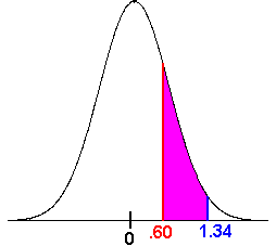
Now we want
P(0.60 < z < 1.34)
This is the "in between" type hence we subtract
P(0.60 < z < 1.34) = P(z < 1.34) - P(z < 0.60)
We use the table to get
P(0.60 < z < 1.34) = .9099 - .7257 = .1842
We conclude that there is about an 18 percent chance that the stress level will be between nine and ten.
Example
Suppose that your wife is pregnant and due in 100 days. Suppose that the probability density distribution function for having a child is approximately normal with mean 100 and standard deviation 8. You have a business trip and will return in 85 days and have to go on another business trip in 107 days.
-
What is the probability that the birth will occur before your second trip?
-
What is the probability that the birth will occur after you return from your first business trip?
-
What is the probability that you will be there for the birth?
-
You are able to cancel your second business trip, and your boss tells you that you can return home from your first trip so that there is a 99% chance that you will make it back for the birth. When must you return home?
Solution:
-
We want
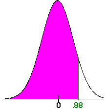
P(x < 107)
We compute the z-score:
107 - 100
z =
8
We computeP(z < .88)
The table on the inside front cover gives usP(z < .88) = .8106
Hence there is about a 81% chance that the baby will be born before the second business trip.
-
We want
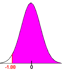
P(x > 85)
We compute the z-score:
85 - 100
z =
8
We compute
P(z > -1.88)
The table on the inside front cover gives us
P(z < -1.88) = .0301
We want the complement of this area hence
P(z > -1.88) = 1 - .0301 = .9699
Hence there is about a 97% chance that the baby will be born after the first business trip.
-
Now we want
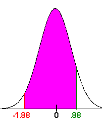
P( 85 < x < 107)
We see form the picture that this is the middle region. We have
P(85 < x < 107) = P(x < 107) - P(x < 85)
We have already computed these. We have
P(85 < x < 107) = P(x < 107) - P(x < 85) = 81% - 3% = 78%
There is about a 78% chance that you will make it to the birth.
This problem asks us to work out the math backwards. We are given the probability and we want the raw score. First, we realize that we if there is a 99% chance that we will make it on time, then there is a 1% chance that we will not. Next, we use the table in reverse. That is, we seek a z-score that gives .01 as the probability.
| z | .00 | .01 | .02 | .03 | .04 | .05 | .06 | .07 | .08 | .09 |
| -2.4 | .0082 | .0080 | .0078 | .0075 | .0073 | .0071 | .0069 | .0068 | .0066 | .0064 |
| -2.3 | .0107 | .0104 | .0102 | .0099 | .0096 | .0094 | .0091 | .0089 | .0087 | .0084 |
| -2.2 | .0139 | .0136 | .0132 | .0129 | .0125 | .0122 | .0119 | .0116 | .0113 | .0110 |
We search for the probability value that is closest to .01 and find .0102 and .0099. Since .0099 is the closest to .01, we use this value. The corresponding z-score is -2.33. Now we find the x that produces this z. We have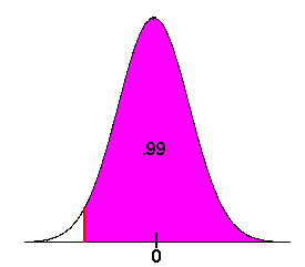
x - 100
-2.33 =
8
Multiply both sides by 8 to get
-18.64 = x - 100
Add 100 to both sides to get
x = 81.36
We must return from our business trip in 81 days.
Using the Normal Distribution to Approximate the Binomial Distribution
The Binomial Distribution is easy to calculate as long as we only need a few values. However, if we need many values, the computation can be extremely tedious.
Example
Suppose you throw a die 1000 times. What is the probability of having it roll a 6 fewer than 160 times?
Solution 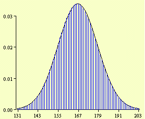
The horrible way of figuring this out is to calculate
C1000,r (1/6)r (5/6)1000 - r
for every r between 0 and 159. We have better things to do with our time than do this. Instead we will approximate the answer. The graph of the distribution is shown on the right. It was created with this program. As you may have already guessed, this distribution is very close to being normal. We give the following theorem
|
Theorem: Normal Approximation to the Binomial Distribution If a binomial distribution with probability of success p and failure q and n trials is such that
Then the distribution can be approximated by a normal distribution with mean m = np and standard deviation
|
Now we can continue with our example.
We have
np = (1000)(1/6) = 166.67 > 5 and nq = (1000)(5/6) = 833 > 5
Thus we can use the normal distribution.
We have
m = np = (1000)(1/6) = 166.67
and
npq = (1000)(1/6)(5/6) = 138.89
Taking a square root gives
s = 11.79
Now we can compute the z-score, since we want P(x < 160). We have
160 - 166.67
z =
= -0.57
11.79
Now we use the table to find the probability. We get .2843. Thus there is about a 28% chance that we will roll a six fewer than 160 times.
Continuity Correction
We can achieve a slightly more accurate approximation with what is called the continuity correction. We looked at P(x < 160). However this is the same as P(x < 159.5) or any such fraction. When using the normal distribution to approximate the binomial distribution, we correct by this .5 value.
Example
Each year a squirrel has a 35% chance of surviving the winter. Suppose in patch of land there are 200 squirrels. What is the probability that between 65 and 80 of these squirrels will survive the winter?
Solution
We first check
np = (200)(.35) = 70 > 5 and nq = (200)(.65) = 130 > 5
Thus we can use the normal curve approximation.
We have
m = np = (200)(.35) = 70
and
npq = (200)(.35)(.65) = 45.5
Taking a square root gives
s = 6.7
Instead of using P(65 < x < 80), we use the continuity correction and find P(64.5 < x < 80.5). We compute the two z-scores.
64.5 - 70
z =
= -.82
6.7
and
80.5 - 70
z =
= 1.57
6.7
Now we use the table to find the probabilities. We get .2061 and .9418. Since we want the middle area, we subtract these
.9418 - .2061 = .7357
Thus there is about a 73% chance that there will be between 65 and 80 surviving squirrels.
Handout of additional examples and exercises
Back to the Probability Home Page
Back to the Elementary Statistics (Math 201) Home Page