Math 201 Practice Midterm 3
Please work out each of the given problems. Credit will be based on the steps that you show towards the final answer. Show your work.
Problem 1
A study was done to determine whether LTCC transfer students had a lower retention rate from the retention rate of the average US student retention rate of 71%. Of the 121 LTCC transfer students tracked, 84 eventually received their bachelor's degree. What can you conclude with a level of significance of 5%? Give the P-value and interpret what it means.
We form the hypotheses
H0: p = .71 H1: p < .71
Since the level of significance is 95%
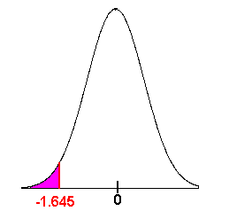
and this is a left tailed test, we use -1.645 for zc.
The observed proportion is 
p = 84/121 = .69
Now we compute the z-score. We have

This does not lie in the critical region, hence we fail to reject the null hypothesis and can conclude that there is insufficient evidence to make a conclusion about retention rates being lower for LTCC transfer students then for the average student. More resources are needed to further investigate the situation.
We look at the table for the P-value. The table gives a value of .3156. This is a large P-value requiring a level of significance of 32% or more in order to reject the null hypothesis.
Problem 2
Thirteen males and fourteen females participated in a study of grip and leg strength. Right leg strength (in Newtons) was recorded for each participant resulting in the table below. Is there a difference between strength in men and women? Use a 5% level of significance. Give the P-value and interpret what it means.
| Gender | n | x | s |
| Male | 13 | 2127 | 513 |
| Female | 14 | 1643 | 446 |
This is a hypothesis of the difference between means. We have
H0: m1 - m2
=
0 H1: m1
- m2
![]() 0
0
Since these are small samples, we calculate the standard error.
![]()
so that
2127 - 1643
t =
= 2.60
186
With 12 degrees of freedom, the P-value is between 0.02 and 0.05. This means that if it were true that the mean strength was the same for men and women, then there would be between 2% and 5% chance that if we randomly selected 13 men and 14 women, we would get a difference that was at least as large as we got from this survey. Since the P-value is less than 0.05, we reject the null hypothesis and accept the alternative hypothesis. We conclude that there is a difference between men and women's leg strength.
Problem 3
Is one ski resort better than another? Data was collected to determine whether the ski resort that was visited had a bearing on how much enjoyment the skier had. The following table shows the data that was collected. What can you conclude at the 5% level?
| Bored | Had an OK time | Had a Great Time | The Best Experience Ever | |
| Heavenly | 7 | 25 | 42 | 4 |
| Sierra-at-Tahoe | 5 | 20 | 30 | 1 |
| Kirkwood | 9 | 12 | 30 | 15 |
We first state the null and alternative hypotheses
H0: Ski resort and enjoyment are independent
H1: Ski resort and enjoyment are dependent
Next we complete the contingency table by filling in the required expected frequencies
| Bored | Had an OK time | Had a Great Time | The Best Experience Ever | Row Total | |
| Heavenly | O
= 7 #1
E = 8 |
O
= 25 #2
E = 22 |
O
= 42 #3
E = 40 |
O
= 4 #4
E = 8 |
78 |
| Sierra-at-Tahoe | O
= 5 #5
E = 6 |
O
= 20 #6
E = 16 |
O
= 30 #7
E = 29 |
O
= 1 #8
E = 6 |
56 |
| Kirkwood | O
= 9 #9
E = 7 |
O
= 12 #10
E = 19 |
O
= 30 #11
E = 34 |
O
= 15 #12
E = 7 |
66 |
| Column Total | 21 | 57 | 102 | 20 | 200 |
Now we use a table to compute the C2 statistic.
| Cell | O | E | (O - E) | (O - E)2 | (O - E)2/E |
| 1 | 7 | 8 | -1 | 1 | 0.125 |
| 2 | 25 | 22 | 3 | 9 | 0.409 |
| 3 | 42 | 40 | 2 | 4 | 0.1 |
| 4 | 4 | 8 | -4 | 16 | 2 |
| 5 | 5 | 6 | -1 | -1 | 0.167 |
| 6 | 20 | 16 | 4 | 16 | 1 |
| 7 | 30 | 29 | 1 | 1 | 0.034 |
| 8 | 1 | 6 | -5 | 25 | 4.167 |
| 9 | 9 | 7 | 2 | 4 | 0.571 |
| 10 | 12 | 19 | -7 | 49 | 2.579 |
| 11 | 30 | 34 | -4 | 16 | 0.471 |
| 12 | 15 | 7 | 8 | 64 | 9.143 |
We now add the numbers from the last column to get
20.766.
The contingency table is of size 3 x 4 so the number of degrees of freedom is
(3 - 1)(4 - 1) = 6 degrees of freedom
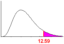
For a = .05, we use the X 2 table and get 12.59. Since 20.766 > 12.59, we can conclude that the ski resort and how much enjoyment a skier experiences are not independent. It does matter which ski resort a skier decides to ski at.
Problem 4
You are the owner of an automobile dealership and have done research on the relationship between the cost of the clothes (x) that a potential buyer wears and the price of the car (y) that the person will buy. 45 different respondents participated in the study. The average customer comes in wearing a $120 outfit. You have found that the equation of the regression line is
y = 8000 + 50x
and that Se = 1000, SSx = 12,000, and n = 45
A. A man walks into your dealership sporting a $200 outfit. What is your prediction for the price of the car that this man will buy?
We just plug in 200 into the regression equation to get
8,000 + 50(200) = 18,000
We can predict that the man will buy a $18,000 car.
B. Find a 95% confidence interval for the price of the car that the man will buy.
We find E

A 95% confidence interval is given by
18,000
![]() 2445
2445
We are 95% confident that the price of the car that this man will buy is between $15,555 and $18,245.
Problem 5
You are the owner of the Tahoe Inn Motel and are interested in how the price per room is related to the number of units that are occupied. Below is the SPSS readout produced from motels throughout the Tahoe area.
A. What is the equation of the regression line? Interpret the slope of the regression line for this study. Interpret the y-intercept.
The equation is
y = 91.4 - 0.52x
The slope tells us that for every $1 that the price is raised, we expect to lose .52 occupants.
The y-intercept tells us that if we allow people to stay in our rooms for free, then we can expect about 91 of our rooms occupied.
B. Use your regression line to provide a point estimate for the number of units occupied when the price per room is $100.
We plug 100 into the equation
y = 91.4 - .52(100) = 39.4
C. What is the correlation coefficient? Interpret this coefficient.
The correlation coefficient is r = -0.69.
We can say that there is a moderate negative correlation between the price per room and occupancy rate.
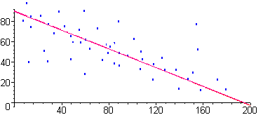
D. Construct a possible scatterplot for this data and explain using a complete sentence or two your reasoning in constructing the scatterplot the way you did it.

There is a general trend downward, but the data do not perfectly fit the regression line.
Simple linear regression results:
Dependent Variable: Units
Independent Variable: Price
Sample size: 26
Correlation coefficient: -0.69
Estimate of sigma: 20.581867
| Parameter | Estimate | Std. Err. | DF | T-Stat | P-Value |
| Intercept | 91.39109 | 6.9450126 | 24 | 13.159241 | <0.0001 |
| Slope | -0.5198245 | 0.111319035 | 24 | -4.669682 | <0.0001 |
Problem 6
Do students do better on exams if they meditate for the hour just before the exam. At a large university the average score on the first exam is 82%. 38 students volunteered to go through an hour of meditation before their first exam. The meditators averaged 84% on the exam with a standard deviation of 5%. What can you conclude at a .05 level? give the P-value and interpret what it means.
The appropriate hypotheses are
H0: m = 82 H1: m > 82
We have
x = 84 s = 5 n = 38
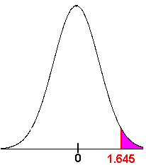
Since we are at a .05 level, the z-critical value is 1.645. We compute the z-score

2.47 falls in the critical region. We can reject the null hypothesis and accept the alternative hypothesis. We can conclude that students who meditate before the exam perform better. We find the P-value by looking at -2.47 in the table. We get
P = .0068
This is a very small P-value, meaning that the data would have been significant even at a smaller (such as .01) level of significance.
Problem 7
A medical researcher is concerned that a new medication has a side effect of raising the variance of the salt content in the blood. For 20 days the blood salinity of a patient who was not on the medication was tested. She calculated the variance as 0.06 percent. Then the patient began taking the medication and the blood salinity was tested for the next 13 days. The variance over these 13 days was found to be 0.15 percent. Use a level of significance of 0.05 to test the claim that the variance of the blood salinity is greater while on medication.
We set up the null and alternative hypothesis:
H0: s12 = s22
H1: s12 < s22
The test statistic is given by
0.15
F =
= 2.50
0.06
The numerator degrees of freedom is 13 - 1 = 12.
The denominator degrees of freedom is 25 - 1 = 24.
We now go to the table and see that 0.025 < P-Value < 0.05 in particular the P-value is less than the level of significance, so we reject the null hypothesis and conclude that the variance in the salinity is greater with the medication than without the medication.
Problem 8
A researcher is interested in determining whether there is a difference between the mean amount of money spent on textbooks in the fall at the three California public university systems. Ten randomly selected students from UC campuses, 8 randomly selected students from Cal State campuses and 14 randomly selected students from community colleges were surveyed. Below is the StatCrunch readout for this survey.
Analysis of Variance results:
Data stored in separate columns.
Column means
| Column | n | Mean | Std. Error |
| UC | 10 | 234.9 | 23.159088 |
| Cal State | 8 | 201.75 | 11.846865 |
| Comm Col | 12 | 183.16667 | 13.26983 |
ANOVA table
| Source | df | SS | MS | F-Stat | P-value |
| Treatments | 2 | 14740.9 | 7370.45 | 2.5071433 | 0.1003 |
| Error | 27 | 79374.07 | 2939.7803 | ||
| Total | 29 | 94114.97 |
A. What assumptions have we made about the data to apply a single-factor ANOVA test?
Solution
Since the data comes from independent random samples, , we need assume only that each group of data came from a normal distribution, and that all the groups came from distributions with about the same standard deviation.
B. What can be concluded at the 0.05 level of significance?
Solution
Since the P-value is 0.1003 is greater than the level of significance of 0.05, we do not have significant evidence to conclude that there is a difference in the mean amount of money spent on textbooks by students at the three institutions.
