Answers for

Review Exam 2, Math 201 (B. Olson)

(NO continuity correction for sections 6.4 and 7.3)

Chapter 5:  The Binomial Distribution

1.  What is the difference between a discrete random variable and a continuous random variable?

A discrete random variable represents countable data, a continuous random variable represents data that is measured.

2.  What is a probability distribution?

A probability distribution has assigned probabilities to each data value or range of values.  The sum of the probabilities in the distribution must equal 1.

3.  What is the expected value of a random variable x in a probability distribution?

The expected value of a random variable x is the mean of the probability distribution. 

Xbar =

4.  What is a binomial experiment?  (Page 221)

A binomial experiment has a fixed number of trials, n.

The n trials are independent and repeated under identical conditions.

Each trial has only two outcomes, success or failure.

For each individual trial, the probability of success is the same, denoted p. 

The probability of failure is 1 – p = q.

The purpose of a binomial experiment is to find the probability of r successes out of n trials.

5.  How do you compute the probabilities for a binomial experiment?

P(r successes out of n trials) = nCr (p)^r (q)^n-r                 where nCr  =

Chapter 6:  The Normal Distribution

1.  What are the properties of a normal curve?  (Page 273)

It is bell-shaped, symmetric about the mean  , the highest point is over the mean , the curve approaches but never touches the horizontal axis, and the transition of the curve from concave up to concave down occurs at  –    and  + .

2.  The normal curve uses what parameters? 

The mean  and the standard deviation .

3.  What is the empirical rule for normal curve?  (Page 276)

68% of the data falls within one standard deviation of the mean on both sides.

95% of the data falls within two standard deviations of the mean on both sides.

99.7% of the data falls within three standard deviations of the mean on both sides.

4.  How do you construct a Control Chart? What are the Out-of-Control Signals?  (Pages 280-281)

Use frequency for the vertical axis.  The time intervals are the horizontal axis.

The mean is a solid horizontal line, the dotted horizontal lines represent two standard deviations and three standard deviations above and below the mean.

Plot the data according to frequency and time interval.

Out-of-control Signal I:  one data point falls beyond the 3 line.

Out-of-control Signal II:  a run of nine consecutive data points fall on the same side of the mean.

Out-of-control Signal III:  at least two out of three consecutive data points fall beyond the 2 line on the same side of the mean.

5.  What are the values of  and  in a Standard Normal Distribution?

 = 0 and  = 1

6.  What is the purpose of a Standard Normal Distribution?

To be able to find the probabilities for ALL normal distributions using the Standard Normal table, without using the function formula.

7.  How do we convert raw scores (x) into Standard units (z-scores) and vice-versa?

z =                                 x = z +

8.  How do we find the area under a standard normal curve given a z value?  (Page 297)

If P(z < z₁ ) then look on the standard normal table (z-table) for the value z₁, the corresponding value is the probability.

If P(z > z₁) then look on the z-table for the value z₁ and subtract that value from 1.

Or use the fact that the normal distribution is symmetrical and find P(z < -z₁) = P(z > z₁).

If P(z₁ < z < z₂) then find P(z < z₂) - P(z < z₁).  Subtract the probabilities.

9.  How do we find a z-value given the probability (or area under the curve)?

Look at the BODY of the z-table for the probability and go out to the left column and the top row for the corresponding z value.

10.  What must be necessary to use a Normal approximation to the Binomial Distribution?

np > 5 AND nq > 5

11.  What are the conversions for the variables needed from the binomial distribution to the standard normal?

np =  and  = 

Chapter 7:  Sampling Distributions

1.  What is the difference between a distribution of a sample and a sampling distribution?

A distribution of a sample is the distribution of one single sample, while a sampling distribution is the distribution of many samples of the same size.

2.  What is a parameter and give examples?

A Parameter is numerical descriptive measure of a population.  , , , p , . . .

3.  What is a statistic and give examples?

A Statistic is a numerical descriptive measure of a sample.  xbar, s, s² , p(hat), . . .

4.  What is Theorem 7.1?  (Page 341)

5.  What is the Central Limit Theorem?  (Page 344)

6.  What makes the Central Limit Theorem different from Theorem 7.1?

For n sufficiently large, the random variable x can have any distribution, and the sampling distribution of xbar will be approximately normal.

7.  What are the conversions for the variables needed in both theorems to convert to a standard normal? (Pages 342 & 345)

                         z =   where n is the sample size

n > 30 for the Central Limit Theorem.

8.  What is the sampling distribution for the proportion p = ?  (Page 353)

9.  What is a P-Chart?  (Pages 358-359)

A control chart for proportions where proportions instead of frequency is graphed

over time intervals.  The mean is now the pooled proportion pbar =

and the standard deviation =

Chapter 8:  Estimation

1.  What is a point estimate?       What is a critical value?

A single number from a sample that estimates a population parameter is a point estimate.

A critical value is the z-value that determines the level of confidence in an estimate.

2.  What is the formula for finding the maximal error tolerance, E in large samples?  (Page 378)

E = z_c         where s = sample standard deviation, z_c is the critical value for a c confidence level, and n is sample size > 30.

3.  What is a confidence interval?

A confidence interval is the range of values that a point estimate will try to be within the population parameter, with a c level of confidence.

4.  Why are we not allowed to use a z variable when estimating the mean with small samples?

If a sample's distribution is not known to be normal, small samples are not enough to approximate the normal distribution, which uses z values.

5.  What distribution is used for estimating the mean for small samples?  What is the formula for the maximal error tolerance?

A Student's t distribution is used for estimating the mean for small samples. 

E = t_c  where t_c is the critical value with c level of confidence and

degrees of freedom = n - 1.   s = sample standard deviation

6.  What formula is used for estimating p in large samples in a Binomial Distribution?

p(hat) - E < p < p(hat) + E      where E = z_c and z_c is the critical value for c level of confidence.

7.  When choosing a sample size for estimating the mean, what are the criteria?

Decide on the level of confidence and the size of the error we are willing to tolerate.

8.  What is the formula to find sample size for estimating the mean?  n =

What about the sample size for estimating p?  n = pq with preliminary estimates for p.

n =  without preliminary estimates for p.

9.  When estimating the difference of means between two populations, what does Theorem 8.1 tell us?  (Page 422)

10.  When finding a c confidence interval for what do we need?

For large samples  (Page 423)              For Small samples  (Page 426)

11.  When finding a c confidence interval for p₁ – p₂ (large samples) what do we need? (Pg. 429)

12.  What does it mean when the difference of two population means is between two positive values?     > 0, so

What if one value is negative and the other is positive?

We cannot form a conclusion about .

Read Chapter Summaries for Sections 5.1 & 5.2 (Pages 260 – 261), Chapter 6 (Pages 324 – 325), Chapter 7 (Pages 364 - 365) and Chapter 8 (Pages 439 – 440).

Go over homework and class notes.

Larry Green has a practice midterm 2 for his class at this website.  Note his second midterm covers different sections.  http://www.ltcconline.net/greenl/courses/201/keys/pMid2.htm

Answers to Review Exam 3 Math 201 (B. Olson)

Chapter 9:

1.  In Hypothesis testing for the mean, what is used for the null hypothesis?  What does the alternate hypothesis intend to show?  What are the notations for each?

The null hypothesis is a specification or long standing claim. H₀:  = k

The alternate hypotheses are either less than, greater than or different from the null hypothesis.         H₁:  < k                        or  H₁:  > k              or  H₁:    k

2.  What is a Type I error?  What notation is used for the probability of this error?

A Type I error is to reject the null hypothesis when it is in fact true. 

is the probability of a Type I error.

3.  What is a Type II error?  What notation is used for the probability of this error?

A Type II error is to fail to reject the null hypothesis when it is in fact false. 

is the probability of a Type II error.

4.  What is the critical region of hypothesis testing?  Where are the critical regions located on the distribution?

The critical region of hypothesis testing is the area under the curve that determines whether or not we reject the null hypothesis.  It is located either at left for a left-tail test, at the right for a right-tail test, or at both ends for a two-tail test.

5.  What is the critical value in testing large samples for the mean?  What is the conversion formula?

 is the critical value associated with the level of significance  for the appropriate tail test for a normal distribution.  The conversion formula for z is

6.   What are the criteria for rejecting or failing to reject the null hypothesis?

If the sample test statistic falls in the critical region, we reject the null hypothesis.  If not, we fail to reject the null hypothesis.

7.  What is a P-value?

A P-value is the smallest probability of making a type I error. 

8.  How do we find the P-value of a hypothesis test?

For a standard normal conversion of z and a one-tail test, look on the table for the z-value and find the probability corresponding to the z-value.  If it is a right tail test, subtract that value from 1.

9.  When looking for the P-value in large sample tests, what must we do for a two-tail test?

How is testing small samples different from large samples?

We must multiply the probability by two in a two-tail test for a normal distribution. 

For testing small samples, the probability has already been accounted for in a Student’s t distribution when looking under  for a two-tail test and the appropriate degrees of freedom.

10.  When testing proportions, what are the null hypothesis and the alternate hypothesis?

H₀ :  p = k, for some k                       H₁ : p < k        or         H₁ : p > k        or         H₁ : p  k

11.  When are we allowed to use the standard normal table and how do we convert to z-values for testing proportions?

If np> 5 AND nq > 5              z =            where q = 1 – p

12.  What is the difference between independent samples and dependent samples?

Independent samples are taken from two populations where the two samples are not related in any way.  The sample sizes taken from each population need not be equal.

Dependent samples are taken from the same object or closely matched items.  These are paired data and must have the same sample size.  The characteristics of each sample should be the same except for the one characteristic being measured.

13.  When testing paired differences, what does dbar represent?

Dbar is the mean (average) difference between two samples means.  

14.  When testing independent sample differences, what are the three types of testing that can occur?

There are differences of two means in large samples, differences of two means in small samples and differences of two proportions.

Chapter 10:

1.  What is a scatter diagram?

A scatter diagram is a graph of points (x, y) taken from paired data.

2.  What does it mean for paired data values to have a linear correlation or not?

Is there a relationship between the x and y values of paired data where a line may come close to representing the paired data?

3.  What are the explanatory variable and the response variable?

The x variable is the explanatory variable and the y variable is the response variable.

4.  What is the Least Squares Criterion?

The sum of the squares of each vertical distance from the actual y value to the predicted y value is the smallest value of any line through the scatter diagram.

5.  What is the equation of the Least Squares Line?  What does each variable represent?

How do we find each part?

y = a + bx                    a = y-intercept                        b = slope of the line               

a = ybar - b(xbar)       b =

6.  What is the Standard Error of the Estimate?

The standard error of the estimate, S_e is the average deviation of the y value from the line of best fit (Least squares line).  It can show how well data fits the line. 

S_e =  where n = the number of data points.

7.  What is the confidence interval for y at a specific value of x?

For a specified c level of confidence, the predicted value of y for a given x is

y_p – E < y < y_p + E     Where E is the error found by t_c S_e

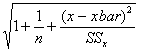
using d.f. = n – 2

8.  What is the Correlation Coefficient r?

The correlation coefficient r, is the measure of how well a scatter diagram correlates to the least squares line. 

9.  What can values of r tell us about the linear correlation if:

a)  r = 0                                                b)  r = 1 or r = -1

a) no linear correlation                      b) perfect linear correlation

c)  0 < r < 1                                         d)  -1 < r < 0

c)  positive low to moderate               d) negative low to moderate correlation

10.  What is an alternate formula for finding the slope of the least squares line?

b = r

11.  What is the Coefficient of determination?  What does it represent?

 r² is the coefficient of determination.

Chapter 11:

1.  How is the Chi-square distribution similar to the Student’s t distribution?  How is it different?

The Chi-square distribution uses degrees of freedom and the test statistic to find the area under curve.  The difference is that the degrees of freedom are not the number in the sample minus one, but either the number of rows and columns are used to find degrees of freedom.

2.  What type of testing uses the Chi-square distribution?

The Chi-square distribution is used in testing independence of two variables and to test the goodness of fit of two distributions.

3.  What are the null hypothesis and the alternate hypothesis of each test?

For Independence: 

H₀: The variables are independent               H₁:  The variables are not independent

For Goodness of Fit:

H₀:  The population fits the given distribution

H₁:  The population does not fit the given distribution.

4.  What is the Observed value vs. the Expected frequency?

The Observed value is the actual collected data from the sample.  The Expected frequency is based on the null hypothesis of independence and what should be the expected amount if independence is true.

5.  What is the formula for finding E in testing independence?

E = expected frequency =  

6.  What is E for testing goodness of fit?

E = expected frequency = (percent of distribution)(sample size)

7.  What is the formula for converting to a value?

=         

Independence: degrees of freedom = (# of rows – 1)(# of columns – 1)

Goodness of fit: degrees of freedom = (# of E entries – 1)

Go over homework problems for Chapters 9, 10, 11.

Larry Green has a practice exam 3 at the website http://www.ltcconline.net/greenl/courses/201/keys/pmid3.htm

Use at your discretion.